Usage

Pymech is a simple interface to read / to write Nek5000 and SIMSON specific data files to / from the Python world. With this capability you could:

• make publication-quality figures

• post-process

• manipulate meshes

• generate initial conditions

• interpolate or extrapolate solution fields, and

possibly many more potential use-cases – the limit is your imagination! Here we look at some simple operations you can do. Start by installing pymech and:

!git clone --recursive https://github.com/eX-Mech/pymech.git
%cd pymech/tests/data/nek

Cloning into 'pymech'...
remote: Enumerating objects: 2443, done.
remote: Counting objects: 100% (794/794), done.
remote: Compressing objects: 100% (291/291), done.
remote: Total 2443 (delta 593), reused 645 (delta 499), pack-reused 1649
Receiving objects: 100% (2443/2443), 12.58 MiB | 37.89 MiB/s, done.
Resolving deltas: 100% (1595/1595), done.
Submodule 'data' (https://github.com/eX-Mech/pymech-test-data.git) registered for path 'tests/data'
Cloning into '/tmp/tmp6yr4pfx7/pymech/tests/data'...
remote: Enumerating objects: 233, done.        
remote: Counting objects: 100% (233/233), done.        
remote: Compressing objects: 100% (151/151), done.        
remote: Total 233 (delta 81), reused 232 (delta 80), pack-reused 0        
Receiving objects: 100% (233/233), 25.70 MiB | 34.71 MiB/s, done.
Resolving deltas: 100% (81/81), done.
Submodule path 'tests/data': checked out '9908c266c7d28ee667a6337ee3cfe73ba577fe3e'
/tmp/tmp6yr4pfx7/pymech/tests/data/nek

pymech.neksuite

from pymech.neksuite import readnek

field = readnek('channel3D_0.f00001')

Simply typing the read field would give you some basic information:

field

<pymech.core.HexaData>
Dimensions:    3
Precision:     4 bytes
Mesh limits:
  * x:         (0.0, 6.2831854820251465)
  * y:         (-1.0, 1.0)
  * z:         (0.0, 3.1415927410125732)
Time:
  * time:      0.2
  * istep:     10
Elements:
  * nel:       512
  * elem:      [<elem centered at [ 0.39269908 -0.98        0.19634954]>
                ...
                <elem centered at [5.89048618 0.98       2.94524309]>]

pymech.core.HexaData

The pymech.core.HexaData class is the in-memory data structure widely used in Pymech. It stores a description of the field and other metadata. Let’s look at the available attributes:

[attr for attr in dir(field) if not attr.startswith('__')]

['check_bcs_present',
 'check_connectivity',
 'elem',
 'elmap',
 'endian',
 'get_points',
 'istep',
 'lims',
 'lr1',
 'merge',
 'nbc',
 'ncurv',
 'ndim',
 'nel',
 'offset_connectivity',
 'time',
 'update_ncurv',
 'var',
 'wdsz']

Here check_connectivity and merge are methods, and elem and elmap are data objects. The rest of the attributes store metadata. See pymech.core to understand what they imply.

print(field.endian, field.istep, field.lr1, field.nbc, field.ncurv, field.ndim, field.nel, field.time, field.var, field.wdsz)

little 10 (8, 8, 8) 0 [] 3 512 0.2 (3, 3, 1, 0, 0) 4

The elem attribute contains data of physical fields. It is an array of lists, with each array representing an element.

print("There are", field.nel, "elements in this file")

There are 512 elements in this file

pymech.core.Elem

The raw arrays are stored as a list of pymech.core.Elem instances as pymech.core.HexaData’s elem attribute.

first_element = field.elem[0]
print("Type =", type(first_element))
print(first_element)

Type = <class 'pymech.core.Elem'>
<elem centered at [ 0.39269908 -0.98        0.19634954]>

Let us look at the attributes of an element

[attr for attr in dir(first_element) if not attr.startswith('__')]

['bcs',
 'ccurv',
 'centroid',
 'curv',
 'face_center',
 'pos',
 'pres',
 'scal',
 'smallest_edge',
 'temp',
 'vel']

Except for the following attributes of an element object

print(first_element.bcs, first_element.ccurv, first_element.curv)

[] ['', '', '', '', '', '', '', '', '', '', '', ''] [[0. 0. 0. 0. 0.]
 [0. 0. 0. 0. 0.]
 [0. 0. 0. 0. 0.]
 [0. 0. 0. 0. 0.]
 [0. 0. 0. 0. 0.]
 [0. 0. 0. 0. 0.]
 [0. 0. 0. 0. 0.]
 [0. 0. 0. 0. 0.]
 [0. 0. 0. 0. 0.]
 [0. 0. 0. 0. 0.]
 [0. 0. 0. 0. 0.]
 [0. 0. 0. 0. 0.]]

it contains large arrays

print("Shape of element velocity and pressure arrays = ", first_element.vel.shape, first_element.pres.shape)

Shape of element velocity and pressure arrays =  (3, 8, 8, 8) (1, 8, 8, 8)

pymech.dataset

from pymech.dataset import open_dataset

ds = open_dataset('channel3D_0.f00001')

This function loads the field file in a more convenient xarray dataset.

ds

<xarray.Dataset>
Dimensions:   (x: 64, y: 64, z: 64)
Coordinates:
  * x         (x) float64 0.0 0.05037 0.1603 0.3105 ... 5.973 6.123 6.233 6.283
  * y         (y) float64 -1.0 -0.9974 -0.9918 -0.9842 ... 0.9918 0.9974 1.0
  * z         (z) float64 0.0 0.02518 0.08017 0.1553 ... 2.986 3.061 3.116 3.142
    time      float64 0.2
Data variables:
    xmesh     (z, y, x) float64 0.0 0.05037 0.1603 0.3105 ... 6.123 6.233 6.283
    ymesh     (z, y, x) float64 -1.0 -1.0 -1.0 -1.0 -1.0 ... 1.0 1.0 1.0 1.0 1.0
    zmesh     (z, y, x) float64 0.0 0.0 0.0 0.0 0.0 ... 3.142 3.142 3.142 3.142
    ux        (z, y, x) float64 0.0 0.0 0.0 0.0 0.0 0.0 ... 0.0 0.0 0.0 0.0 0.0
    uy        (z, y, x) float64 0.0 0.0 0.0 0.0 0.0 0.0 ... 0.0 0.0 0.0 0.0 0.0
    uz        (z, y, x) float64 0.0 0.0 0.0 0.0 0.0 0.0 ... 0.0 0.0 0.0 0.0 0.0
    pressure  (z, y, x) float64 0.004913 0.0467 0.0195 ... 0.03768 0.0761

xarray.Dataset

• Dimensions:
  • x: 64
  • y: 64
  • z: 64
• Coordinates: (4)
  • x
    (x)
    float64
    0.0 0.05037 0.1603 ... 6.233 6.283

    array([0.      , 0.050368, 0.160339, 0.310507, 0.474891, 0.625059, 0.735031,
           0.785398, 0.785398, 0.835766, 0.945737, 1.095906, 1.260289, 1.410457,
           1.520429, 1.570796, 1.570796, 1.621164, 1.731135, 1.881304, 2.045687,
           2.195856, 2.305827, 2.356194, 2.356194, 2.406562, 2.516533, 2.666702,
           2.831085, 2.981254, 3.091225, 3.141593, 3.141593, 3.19196 , 3.301932,
           3.4521  , 3.616483, 3.766652, 3.876623, 3.926991, 3.926991, 3.977358,
           4.08733 , 4.237498, 4.401882, 4.55205 , 4.662022, 4.712389, 4.712389,
           4.762756, 4.872728, 5.022896, 5.18728 , 5.337448, 5.44742 , 5.497787,
           5.497787, 5.548155, 5.658126, 5.808295, 5.972678, 6.122846, 6.232818,
           6.283185])

  • y
    (y)
    float64
    -1.0 -0.9974 -0.9918 ... 0.9974 1.0

    array([-1.      , -0.997435, -0.991834, -0.984186, -0.975814, -0.968166,
           -0.962565, -0.96    , -0.96    , -0.946533, -0.917129, -0.876976,
           -0.833024, -0.792871, -0.763467, -0.75    , -0.75    , -0.730761,
           -0.688755, -0.631395, -0.568605, -0.511245, -0.469239, -0.45    ,
           -0.45    , -0.421142, -0.358133, -0.272092, -0.177908, -0.091867,
           -0.028858,  0.      ,  0.      ,  0.028858,  0.091867,  0.177908,
            0.272092,  0.358133,  0.421142,  0.45    ,  0.45    ,  0.469239,
            0.511245,  0.568605,  0.631395,  0.688755,  0.730761,  0.75    ,
            0.75    ,  0.763467,  0.792871,  0.833024,  0.876976,  0.917129,
            0.946533,  0.96    ,  0.96    ,  0.962565,  0.968166,  0.975814,
            0.984186,  0.991834,  0.997435,  1.      ])

  • z
    (z)
    float64
    0.0 0.02518 0.08017 ... 3.116 3.142

    array([0.      , 0.025184, 0.080169, 0.155254, 0.237445, 0.31253 , 0.367515,
           0.392699, 0.392699, 0.417883, 0.472869, 0.547953, 0.630144, 0.705229,
           0.760214, 0.785398, 0.785398, 0.810582, 0.865568, 0.940652, 1.022843,
           1.097928, 1.152913, 1.178097, 1.178097, 1.203281, 1.258267, 1.333351,
           1.415543, 1.490627, 1.545613, 1.570796, 1.570796, 1.59598 , 1.650966,
           1.72605 , 1.808242, 1.883326, 1.938312, 1.963495, 1.963495, 1.988679,
           2.043665, 2.118749, 2.200941, 2.276025, 2.331011, 2.356194, 2.356194,
           2.381378, 2.436364, 2.511448, 2.59364 , 2.668724, 2.72371 , 2.748893,
           2.748893, 2.774077, 2.829063, 2.904147, 2.986339, 3.061423, 3.116409,
           3.141593])

  • time
    ()
    float64
    0.2

    array(0.2)

• Data variables: (7)
  • xmesh
    (z, y, x)
    float64
    0.0 0.05037 0.1603 ... 6.233 6.283

    array([[[0.        , 0.05036753, 0.16033897, ..., 6.12284613,
             6.23281765, 6.28318548],
            [0.        , 0.05036753, 0.16033897, ..., 6.12284613,
             6.23281765, 6.28318548],
            [0.        , 0.05036753, 0.16033897, ..., 6.12284613,
             6.23281765, 6.28318548],
            ...,
            [0.        , 0.05036753, 0.16033897, ..., 6.12284613,
             6.23281765, 6.28318548],
            [0.        , 0.05036753, 0.16033897, ..., 6.12284613,
             6.23281765, 6.28318548],
            [0.        , 0.05036753, 0.16033897, ..., 6.12284613,
             6.23281765, 6.28318548]],
    
           [[0.        , 0.05036753, 0.16033897, ..., 6.12284613,
             6.23281765, 6.28318548],
            [0.        , 0.05036753, 0.16033897, ..., 6.12284613,
             6.23281765, 6.28318548],
            [0.        , 0.05036753, 0.16033897, ..., 6.12284613,
             6.23281765, 6.28318548],
    ...
            [0.        , 0.05036753, 0.16033897, ..., 6.12284613,
             6.23281765, 6.28318548],
            [0.        , 0.05036753, 0.16033897, ..., 6.12284613,
             6.23281765, 6.28318548],
            [0.        , 0.05036753, 0.16033897, ..., 6.12284613,
             6.23281765, 6.28318548]],
    
           [[0.        , 0.05036753, 0.16033897, ..., 6.12284613,
             6.23281765, 6.28318548],
            [0.        , 0.05036753, 0.16033897, ..., 6.12284613,
             6.23281765, 6.28318548],
            [0.        , 0.05036753, 0.16033897, ..., 6.12284613,
             6.23281765, 6.28318548],
            ...,
            [0.        , 0.05036753, 0.16033897, ..., 6.12284613,
             6.23281765, 6.28318548],
            [0.        , 0.05036753, 0.16033897, ..., 6.12284613,
             6.23281765, 6.28318548],
            [0.        , 0.05036753, 0.16033897, ..., 6.12284613,
             6.23281765, 6.28318548]]])

  • ymesh
    (z, y, x)
    float64
    -1.0 -1.0 -1.0 -1.0 ... 1.0 1.0 1.0

    array([[[-1.        , -1.        , -1.        , ..., -1.        ,
             -1.        , -1.        ],
            [-0.99743479, -0.99743479, -0.99743479, ..., -0.99743479,
             -0.99743479, -0.99743479],
            [-0.99183398, -0.99183398, -0.99183398, ..., -0.99183398,
             -0.99183398, -0.99183398],
            ...,
            [ 0.99183398,  0.99183398,  0.99183398, ...,  0.99183398,
              0.99183398,  0.99183398],
            [ 0.99743479,  0.99743479,  0.99743479, ...,  0.99743479,
              0.99743479,  0.99743479],
            [ 1.        ,  1.        ,  1.        , ...,  1.        ,
              1.        ,  1.        ]],
    
           [[-1.        , -1.        , -1.        , ..., -1.        ,
             -1.        , -1.        ],
            [-0.99743479, -0.99743479, -0.99743479, ..., -0.99743479,
             -0.99743479, -0.99743479],
            [-0.99183398, -0.99183398, -0.99183398, ..., -0.99183398,
             -0.99183398, -0.99183398],
    ...
            [ 0.99183398,  0.99183398,  0.99183398, ...,  0.99183398,
              0.99183398,  0.99183398],
            [ 0.99743479,  0.99743479,  0.99743479, ...,  0.99743479,
              0.99743479,  0.99743479],
            [ 1.        ,  1.        ,  1.        , ...,  1.        ,
              1.        ,  1.        ]],
    
           [[-1.        , -1.        , -1.        , ..., -1.        ,
             -1.        , -1.        ],
            [-0.99743479, -0.99743479, -0.99743479, ..., -0.99743479,
             -0.99743479, -0.99743479],
            [-0.99183398, -0.99183398, -0.99183398, ..., -0.99183398,
             -0.99183398, -0.99183398],
            ...,
            [ 0.99183398,  0.99183398,  0.99183398, ...,  0.99183398,
              0.99183398,  0.99183398],
            [ 0.99743479,  0.99743479,  0.99743479, ...,  0.99743479,
              0.99743479,  0.99743479],
            [ 1.        ,  1.        ,  1.        , ...,  1.        ,
              1.        ,  1.        ]]])

  • zmesh
    (z, y, x)
    float64
    0.0 0.0 0.0 ... 3.142 3.142 3.142

    array([[[0.        , 0.        , 0.        , ..., 0.        ,
             0.        , 0.        ],
            [0.        , 0.        , 0.        , ..., 0.        ,
             0.        , 0.        ],
            [0.        , 0.        , 0.        , ..., 0.        ,
             0.        , 0.        ],
            ...,
            [0.        , 0.        , 0.        , ..., 0.        ,
             0.        , 0.        ],
            [0.        , 0.        , 0.        , ..., 0.        ,
             0.        , 0.        ],
            [0.        , 0.        , 0.        , ..., 0.        ,
             0.        , 0.        ]],
    
           [[0.02518376, 0.02518376, 0.02518376, ..., 0.02518376,
             0.02518376, 0.02518376],
            [0.02518376, 0.02518376, 0.02518376, ..., 0.02518376,
             0.02518376, 0.02518376],
            [0.02518376, 0.02518376, 0.02518376, ..., 0.02518376,
             0.02518376, 0.02518376],
    ...
            [3.11640882, 3.11640882, 3.11640882, ..., 3.11640882,
             3.11640882, 3.11640882],
            [3.11640882, 3.11640882, 3.11640882, ..., 3.11640882,
             3.11640882, 3.11640882],
            [3.11640882, 3.11640882, 3.11640882, ..., 3.11640882,
             3.11640882, 3.11640882]],
    
           [[3.14159274, 3.14159274, 3.14159274, ..., 3.14159274,
             3.14159274, 3.14159274],
            [3.14159274, 3.14159274, 3.14159274, ..., 3.14159274,
             3.14159274, 3.14159274],
            [3.14159274, 3.14159274, 3.14159274, ..., 3.14159274,
             3.14159274, 3.14159274],
            ...,
            [3.14159274, 3.14159274, 3.14159274, ..., 3.14159274,
             3.14159274, 3.14159274],
            [3.14159274, 3.14159274, 3.14159274, ..., 3.14159274,
             3.14159274, 3.14159274],
            [3.14159274, 3.14159274, 3.14159274, ..., 3.14159274,
             3.14159274, 3.14159274]]])

  • ux
    (z, y, x)
    float64
    0.0 0.0 0.0 0.0 ... 0.0 0.0 0.0 0.0

    array([[[0.        , 0.        , 0.        , ..., 0.        ,
             0.        , 0.        ],
            [0.00782399, 0.01109818, 0.01232493, ..., 0.01113664,
             0.00924522, 0.00782399],
            [0.02854787, 0.03596754, 0.0375705 , ..., 0.03586552,
             0.02966127, 0.02854787],
            ...,
            [0.03577859, 0.04090307, 0.03286156, ..., 0.03289541,
             0.03026278, 0.03577859],
            [0.01168688, 0.01325105, 0.00995309, ..., 0.00990848,
             0.00882348, 0.01168688],
            [0.        , 0.        , 0.        , ..., 0.        ,
             0.        , 0.        ]],
    
           [[0.        , 0.        , 0.        , ..., 0.        ,
             0.        , 0.        ],
            [0.00862066, 0.01083499, 0.01300981, ..., 0.01177836,
             0.00767483, 0.00862066],
            [0.02948931, 0.0353213 , 0.03967586, ..., 0.03711158,
             0.02684145, 0.02948931],
    ...
            [0.03198694, 0.03879612, 0.03513152, ..., 0.0356083 ,
             0.03377092, 0.03198694],
            [0.00972235, 0.01265919, 0.01098284, ..., 0.01119736,
             0.01011113, 0.00972235],
            [0.        , 0.        , 0.        , ..., 0.        ,
             0.        , 0.        ]],
    
           [[0.        , 0.        , 0.        , ..., 0.        ,
             0.        , 0.        ],
            [0.00782399, 0.01109818, 0.01232493, ..., 0.01113664,
             0.00924522, 0.00782399],
            [0.02854787, 0.03596754, 0.0375705 , ..., 0.03586552,
             0.02966127, 0.02854787],
            ...,
            [0.03577859, 0.04090307, 0.03286156, ..., 0.03289541,
             0.03026278, 0.03577859],
            [0.01168688, 0.01325105, 0.00995309, ..., 0.00990848,
             0.00882348, 0.01168688],
            [0.        , 0.        , 0.        , ..., 0.        ,
             0.        , 0.        ]]])

  • uy
    (z, y, x)
    float64
    0.0 0.0 0.0 0.0 ... 0.0 0.0 0.0 0.0

    array([[[ 0.00000000e+00,  0.00000000e+00,  0.00000000e+00, ...,
              0.00000000e+00,  0.00000000e+00,  0.00000000e+00],
            [ 5.86162601e-03, -5.18644229e-04, -1.12613512e-03, ...,
             -3.26120527e-03,  3.27435392e-03,  5.86162601e-03],
            [ 1.29187107e-02, -4.15467686e-04, -2.70633772e-03, ...,
             -8.00271612e-03,  6.89876080e-03,  1.29187107e-02],
            ...,
            [-7.42084999e-03,  2.83849426e-03,  4.15616110e-03, ...,
              4.13650088e-03,  1.36244972e-03, -7.42084999e-03],
            [-3.67996399e-03,  1.35924621e-03,  1.12457632e-03, ...,
              2.18887930e-03,  5.09342062e-04, -3.67996399e-03],
            [ 0.00000000e+00,  0.00000000e+00,  0.00000000e+00, ...,
              0.00000000e+00,  0.00000000e+00,  0.00000000e+00]],
    
           [[ 0.00000000e+00,  0.00000000e+00,  0.00000000e+00, ...,
              0.00000000e+00,  0.00000000e+00,  0.00000000e+00],
            [ 4.81717521e-03,  4.24871081e-03,  9.01214880e-05, ...,
             -5.18017355e-03, -8.70640390e-04,  4.81717521e-03],
            [ 1.08530046e-02,  9.34212003e-03, -4.07323416e-04, ...,
             -1.21738976e-02, -1.76981511e-03,  1.08530046e-02],
    ...
            [ 3.57413990e-03, -1.24165020e-03,  4.92485194e-03, ...,
             -1.63427135e-03,  7.14732008e-03,  3.57413990e-03],
            [ 1.33595592e-03, -7.81269104e-04,  2.24559102e-03, ...,
             -7.50326435e-04,  3.06352321e-03,  1.33595592e-03],
            [ 0.00000000e+00,  0.00000000e+00,  0.00000000e+00, ...,
              0.00000000e+00,  0.00000000e+00,  0.00000000e+00]],
    
           [[ 0.00000000e+00,  0.00000000e+00,  0.00000000e+00, ...,
              0.00000000e+00,  0.00000000e+00,  0.00000000e+00],
            [ 5.86162601e-03, -5.18644229e-04, -1.12613512e-03, ...,
             -3.26120527e-03,  3.27435392e-03,  5.86162601e-03],
            [ 1.29187107e-02, -4.15467686e-04, -2.70633772e-03, ...,
             -8.00271612e-03,  6.89876080e-03,  1.29187107e-02],
            ...,
            [-7.42084999e-03,  2.83849426e-03,  4.15616110e-03, ...,
              4.13650088e-03,  1.36244972e-03, -7.42084999e-03],
            [-3.67996399e-03,  1.35924621e-03,  1.12457632e-03, ...,
              2.18887930e-03,  5.09342062e-04, -3.67996399e-03],
            [ 0.00000000e+00,  0.00000000e+00,  0.00000000e+00, ...,
              0.00000000e+00,  0.00000000e+00,  0.00000000e+00]]])

  • uz
    (z, y, x)
    float64
    0.0 0.0 0.0 0.0 ... 0.0 0.0 0.0 0.0

    array([[[ 0.00000000e+00,  0.00000000e+00,  0.00000000e+00, ...,
              0.00000000e+00,  0.00000000e+00,  0.00000000e+00],
            [-2.57243239e-03, -2.61909026e-03, -2.86152656e-03, ...,
              1.10847724e-03, -1.50612253e-03, -2.57243239e-03],
            [-6.46327995e-03, -6.92148553e-03, -4.93503781e-03, ...,
              5.01798932e-03, -2.32643588e-03, -6.46327995e-03],
            ...,
            [-6.45538839e-03,  4.35915962e-03,  3.93884664e-04, ...,
              9.55819618e-03, -4.59259190e-03, -6.45538839e-03],
            [-2.17044447e-03,  2.52539315e-03,  8.08421464e-05, ...,
              4.20754636e-03, -1.35930558e-03, -2.17044447e-03],
            [ 0.00000000e+00,  0.00000000e+00,  0.00000000e+00, ...,
              0.00000000e+00,  0.00000000e+00,  0.00000000e+00]],
    
           [[ 0.00000000e+00,  0.00000000e+00,  0.00000000e+00, ...,
              0.00000000e+00,  0.00000000e+00,  0.00000000e+00],
            [-4.98422375e-03, -4.73099388e-03, -3.95468855e-03, ...,
              3.13721248e-03, -2.63006729e-03, -4.98422375e-03],
            [-8.94245133e-03, -1.02904793e-02, -8.48434307e-03, ...,
              6.03608927e-03, -3.65531980e-03, -8.94245133e-03],
    ...
            [-3.01487395e-03,  2.87191221e-03, -1.42062898e-03, ...,
              1.24280713e-02, -1.93443871e-03, -3.01487395e-03],
            [-1.20018388e-03,  1.48797024e-03, -1.41262868e-03, ...,
              5.65800397e-03, -1.18875410e-03, -1.20018388e-03],
            [ 0.00000000e+00,  0.00000000e+00,  0.00000000e+00, ...,
              0.00000000e+00,  0.00000000e+00,  0.00000000e+00]],
    
           [[ 0.00000000e+00,  0.00000000e+00,  0.00000000e+00, ...,
              0.00000000e+00,  0.00000000e+00,  0.00000000e+00],
            [-2.57243239e-03, -2.61909026e-03, -2.86152656e-03, ...,
              1.10847724e-03, -1.50612253e-03, -2.57243239e-03],
            [-6.46327995e-03, -6.92148553e-03, -4.93503781e-03, ...,
              5.01798932e-03, -2.32643588e-03, -6.46327995e-03],
            ...,
            [-6.45538839e-03,  4.35915962e-03,  3.93884664e-04, ...,
              9.55819618e-03, -4.59259190e-03, -6.45538839e-03],
            [-2.17044447e-03,  2.52539315e-03,  8.08421464e-05, ...,
              4.20754636e-03, -1.35930558e-03, -2.17044447e-03],
            [ 0.00000000e+00,  0.00000000e+00,  0.00000000e+00, ...,
              0.00000000e+00,  0.00000000e+00,  0.00000000e+00]]])

  • pressure
    (z, y, x)
    float64
    0.004913 0.0467 ... 0.03768 0.0761

    array([[[ 0.00491315,  0.04670352,  0.01950169, ..., -0.01318173,
             -0.0448321 ,  0.00491315],
            [-0.00244926,  0.04848084,  0.02026715, ..., -0.01109768,
             -0.04885662, -0.00244926],
            [-0.00911038,  0.04843532,  0.02007361, ..., -0.01043648,
             -0.04885925, -0.00911038],
            ...,
            [ 0.0575432 ,  0.01674989,  0.06237574, ..., -0.08608513,
              0.03453081,  0.0575432 ],
            [ 0.06938265,  0.01581831,  0.07163108, ..., -0.09748867,
              0.03736472,  0.06938265],
            [ 0.0760996 ,  0.0141098 ,  0.07509886, ..., -0.10274781,
              0.03767838,  0.0760996 ]],
    
           [[ 0.07571961,  0.10852831,  0.09428115, ..., -0.03461239,
              0.01407335,  0.07571961],
            [ 0.06964236,  0.10226395,  0.09199718, ..., -0.02951211,
              0.01538557,  0.06964236],
            [ 0.06034465,  0.09097896,  0.08381573, ..., -0.02420055,
              0.01669309,  0.06034465],
    ...
            [ 0.07753077,  0.05483663,  0.02600924, ..., -0.0315371 ,
              0.03526619,  0.07753077],
            [ 0.08487762,  0.06042636,  0.02248098, ..., -0.03169889,
              0.03567362,  0.08487762],
            [ 0.08565937,  0.06280785,  0.01944153, ..., -0.03090431,
              0.03322716,  0.08565937]],
    
           [[ 0.00491315,  0.04670352,  0.01950169, ..., -0.01318173,
             -0.0448321 ,  0.00491315],
            [-0.00244926,  0.04848084,  0.02026715, ..., -0.01109768,
             -0.04885662, -0.00244926],
            [-0.00911038,  0.04843532,  0.02007361, ..., -0.01043648,
             -0.04885925, -0.00911038],
            ...,
            [ 0.0575432 ,  0.01674989,  0.06237574, ..., -0.08608513,
              0.03453081,  0.0575432 ],
            [ 0.06938265,  0.01581831,  0.07163108, ..., -0.09748867,
              0.03736472,  0.06938265],
            [ 0.0760996 ,  0.0141098 ,  0.07509886, ..., -0.10274781,
              0.03767838,  0.0760996 ]]])

• Attributes: (0)

The dataset is more descriptive and useful for exploratory work, such as post-processing and plotting.

Computing statistics

Calculate median for all variables

ds.median()

<xarray.Dataset>
Dimensions:   ()
Coordinates:
    time      float64 0.2
Data variables:
    xmesh     float64 3.142
    ymesh     float64 0.0
    zmesh     float64 1.571
    ux        float64 0.8375
    uy        float64 0.0
    uz        float64 0.0
    pressure  float64 0.0001238

xarray.Dataset

• Dimensions:
• Coordinates: (1)
  • time
    ()
    float64
    0.2

    array(0.2)

• Data variables: (7)
  • xmesh
    ()
    float64
    3.142

    array(3.14159274)

  • ymesh
    ()
    float64
    0.0

    array(0.)

  • zmesh
    ()
    float64
    1.571

    array(1.57079637)

  • ux
    ()
    float64
    0.8375

    array(0.83750063)

  • uy
    ()
    float64
    0.0

    array(0.)

  • uz
    ()
    float64
    0.0

    array(0.)

  • pressure
    ()
    float64
    0.0001238

    array(0.00012376)

• Attributes: (0)

Slicing

Slice by index:

ds.ux.isel(z=32)

<xarray.DataArray 'ux' (y: 64, x: 64)>
array([[0.        , 0.        , 0.        , ..., 0.        , 0.        ,
        0.        ],
       [0.006773  , 0.01130644, 0.01251847, ..., 0.01209086, 0.01235788,
        0.006773  ],
       [0.02467888, 0.03595118, 0.03948131, ..., 0.03794473, 0.03727177,
        0.02467888],
       ...,
       [0.03804531, 0.0281054 , 0.03863081, ..., 0.03893135, 0.04252424,
        0.03804531],
       [0.01240053, 0.00786791, 0.01261182, ..., 0.01296887, 0.01406241,
        0.01240053],
       [0.        , 0.        , 0.        , ..., 0.        , 0.        ,
        0.        ]])
Coordinates:
  * x        (x) float64 0.0 0.05037 0.1603 0.3105 ... 5.973 6.123 6.233 6.283
  * y        (y) float64 -1.0 -0.9974 -0.9918 -0.9842 ... 0.9918 0.9974 1.0
    z        float64 1.571
    time     float64 0.2

xarray.DataArray

'ux'

• y: 64
• x: 64

• 0.0 0.0 0.0 0.0 0.0 0.0 0.0 0.0 ... 0.0 0.0 0.0 0.0 0.0 0.0 0.0 0.0

  array([[0.        , 0.        , 0.        , ..., 0.        , 0.        ,
          0.        ],
         [0.006773  , 0.01130644, 0.01251847, ..., 0.01209086, 0.01235788,
          0.006773  ],
         [0.02467888, 0.03595118, 0.03948131, ..., 0.03794473, 0.03727177,
          0.02467888],
         ...,
         [0.03804531, 0.0281054 , 0.03863081, ..., 0.03893135, 0.04252424,
          0.03804531],
         [0.01240053, 0.00786791, 0.01261182, ..., 0.01296887, 0.01406241,
          0.01240053],
         [0.        , 0.        , 0.        , ..., 0.        , 0.        ,
          0.        ]])

• Coordinates: (4)
  • x
    (x)
    float64
    0.0 0.05037 0.1603 ... 6.233 6.283

    array([0.      , 0.050368, 0.160339, 0.310507, 0.474891, 0.625059, 0.735031,
           0.785398, 0.785398, 0.835766, 0.945737, 1.095906, 1.260289, 1.410457,
           1.520429, 1.570796, 1.570796, 1.621164, 1.731135, 1.881304, 2.045687,
           2.195856, 2.305827, 2.356194, 2.356194, 2.406562, 2.516533, 2.666702,
           2.831085, 2.981254, 3.091225, 3.141593, 3.141593, 3.19196 , 3.301932,
           3.4521  , 3.616483, 3.766652, 3.876623, 3.926991, 3.926991, 3.977358,
           4.08733 , 4.237498, 4.401882, 4.55205 , 4.662022, 4.712389, 4.712389,
           4.762756, 4.872728, 5.022896, 5.18728 , 5.337448, 5.44742 , 5.497787,
           5.497787, 5.548155, 5.658126, 5.808295, 5.972678, 6.122846, 6.232818,
           6.283185])

  • y
    (y)
    float64
    -1.0 -0.9974 -0.9918 ... 0.9974 1.0

    array([-1.      , -0.997435, -0.991834, -0.984186, -0.975814, -0.968166,
           -0.962565, -0.96    , -0.96    , -0.946533, -0.917129, -0.876976,
           -0.833024, -0.792871, -0.763467, -0.75    , -0.75    , -0.730761,
           -0.688755, -0.631395, -0.568605, -0.511245, -0.469239, -0.45    ,
           -0.45    , -0.421142, -0.358133, -0.272092, -0.177908, -0.091867,
           -0.028858,  0.      ,  0.      ,  0.028858,  0.091867,  0.177908,
            0.272092,  0.358133,  0.421142,  0.45    ,  0.45    ,  0.469239,
            0.511245,  0.568605,  0.631395,  0.688755,  0.730761,  0.75    ,
            0.75    ,  0.763467,  0.792871,  0.833024,  0.876976,  0.917129,
            0.946533,  0.96    ,  0.96    ,  0.962565,  0.968166,  0.975814,
            0.984186,  0.991834,  0.997435,  1.      ])

  • z
    ()
    float64
    1.571

    array(1.57079637)

  • time
    ()
    float64
    0.2

    array(0.2)

• Attributes: (0)

It is also possible to slice by value using sel method

Visualizing

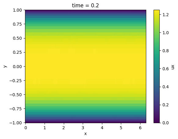
Average in spanwise (z) direction and plot velocity profile

ds.ux.mean('z').plot()

<matplotlib.collections.QuadMesh at 0x7fc5a179b590>

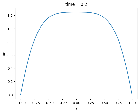
Average in both horizontal direction and plot 1D profile

ds_1d = ds.mean(['x', 'z'])
ds_1d.ux.plot()

[<matplotlib.lines.Line2D at 0x7fc59e71fd90>]

It is also worth knowing that it is possible to:

• Parallelize these operations using ds.chunk method followed by ds.compute

• Open a multiple files into a single dataset using pymech.dataset.open_mfdataset, optionally in parallel.

Read the xarray documentation to see how to use them.